
Method
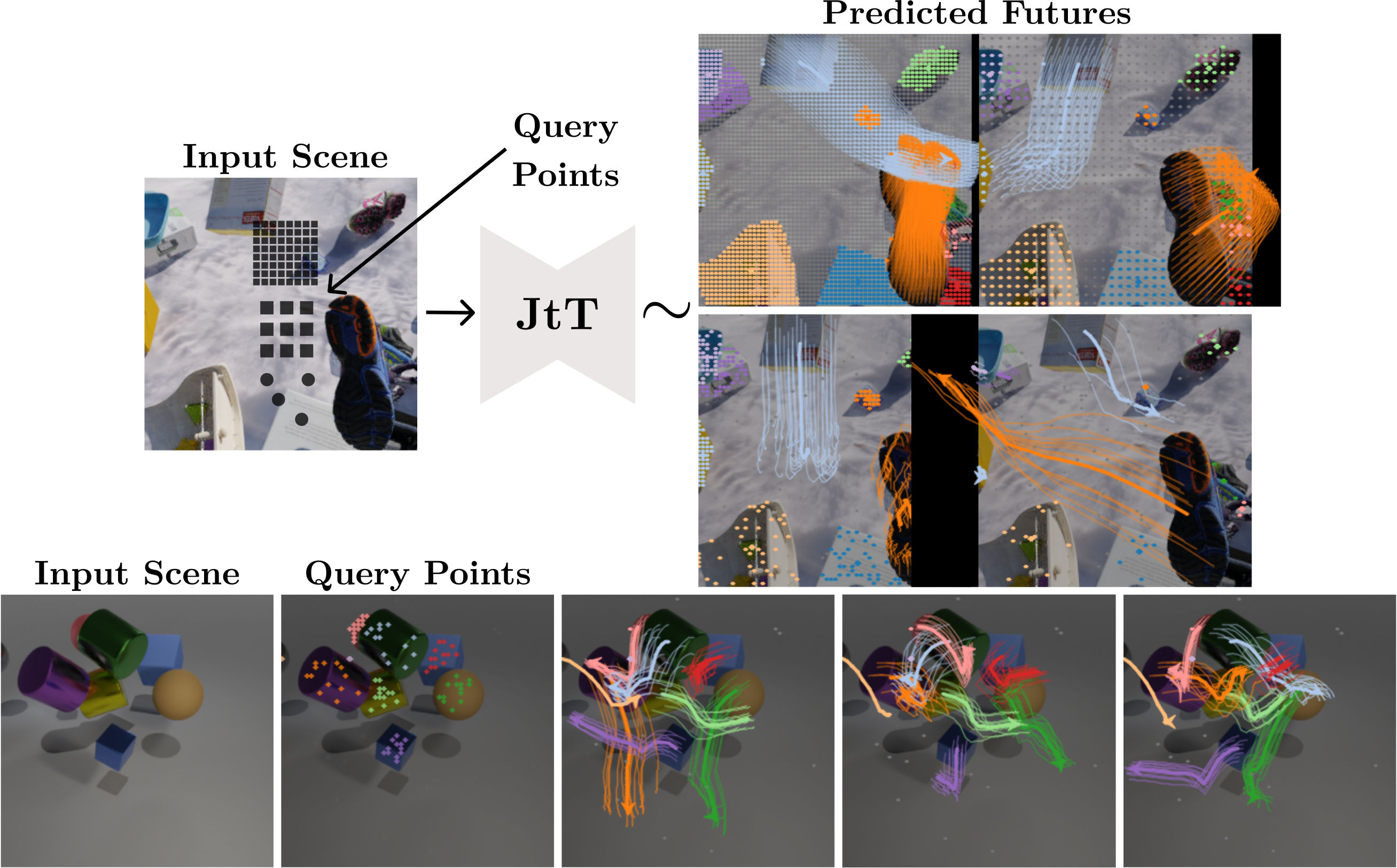
A trajectory is a sequence \(\boldsymbol{x} = (x_0, \dots, x_T)\) of 2D points that starts at a query location \(q = x_0\). Given an image \(I\) and \(N\) query points \(\mathcal{Q} = \{q_n\}_{n=1}^N\), the model samples trajectories from the conditional distribution \(p(\{\boldsymbol{x}_n\}_{n=1}^N \mid I, \mathcal{Q})\).Compared with prior work, the query set \(\mathcal{Q}\) is supplied at inference rather than fixed, and the model is given only the image as evidence: no goal frame, segmentation, depth, or correspondences. Since an image does not fully determine the state of the scene, many futures are possible, and a useful predictor must capture their distribution rather than a single realization.
JtT, the Just trajectory Transformer, is a single diffusion transformer that operates directly in coordinate space. It is generative, sampling multiple distinct futures per scene; flexible, accepting any number of query points at arbitrary locations; and dense, scaling to thousands of points per scene on a single GPU. The design is deliberately minimal,No VAE, auxiliary losses, rollout fine-tuning, or pre-trained video latents are used. The S model has about \(50\)M parameters. but four choices turn out to be critical: what to diffuse, how to inject visual information, which timestep schedule to use, and how to partition the query tokens.
What to diffuse
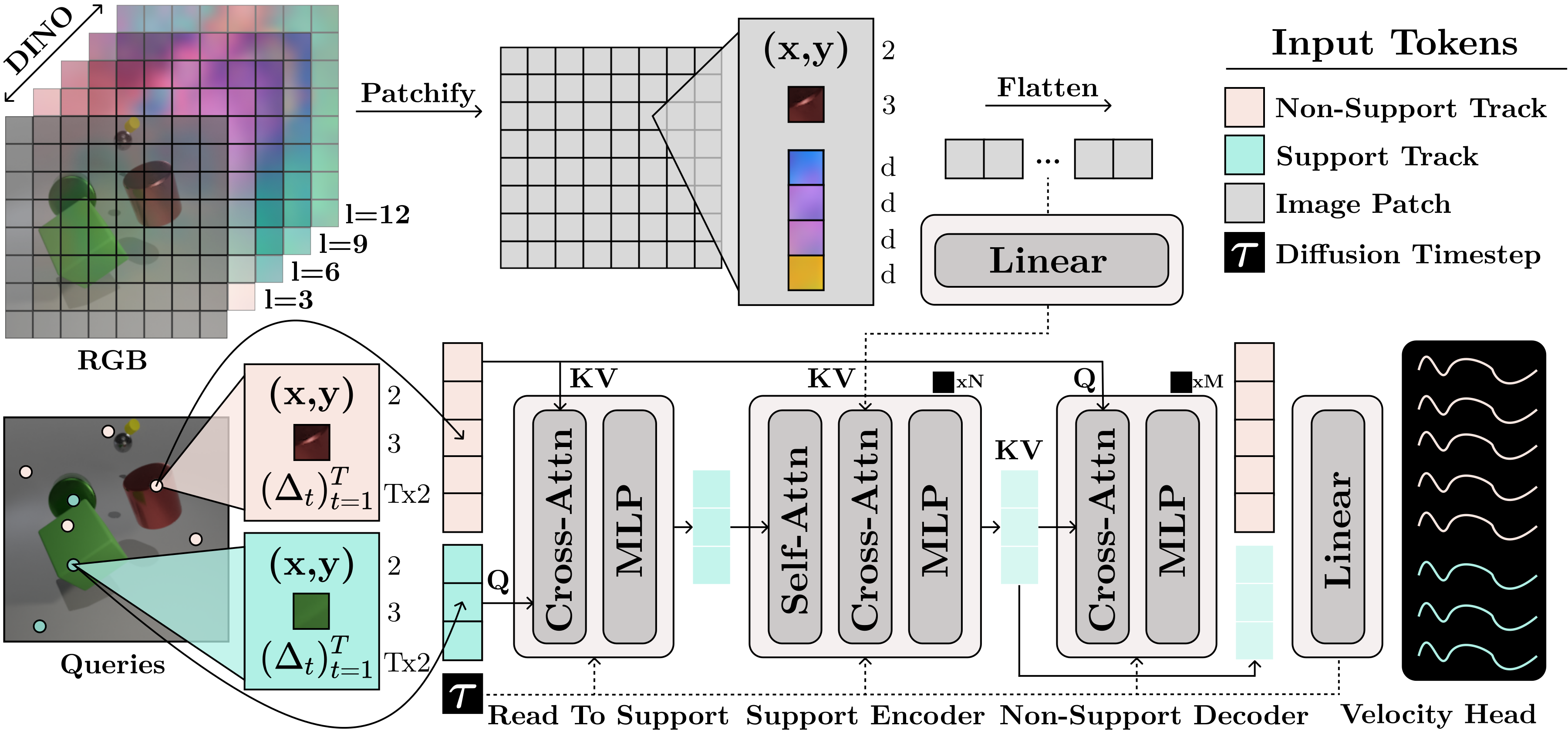
Each trajectory is parameterized as the sequence of instantaneous velocities \(\Delta_t \equiv x_t - x_{t-1}\), and these are the diffusion target.Velocities are isotropically normalized across the dataset so the diffusion target has roughly unit variance. The trajectory is recovered at inference as \(x_t = q + \sum_{i=1}^{t} \Delta_i\). Compared with absolute coordinates \(x_t\), which couple the target to the query location, and grid-cell offsets \(x_t - x_c\), which assume a fixed inference grid, per-frame velocities are translation-equivariant in the query, lie on a near-zero, dataset-normalized scale, and decouple the trajectory from the pixel grid.
The model is trained with a rectified-flow objective on the linear path \(\Delta_\tau = (1-\tau)\,\Delta_0 + \tau\,\Delta_1\), with \(\Delta_0 \sim \mathcal{N}(0, I)\): $$\mathcal{L}(\theta) = \mathbb{E}\left[\,\big\|\hat{\boldsymbol{v}}_\theta(\Delta_\tau, I, \mathcal{Q}, \tau) - (\Delta_1 - \Delta_0)\big\|_2^2\,\right].$$ The timestep \(\tau\) is sampled from a logit-normal distribution rather than uniformly. A uniform schedule overfits the single observed future per initial condition, whereas logit-normal sampling up-weights mid-noise levels and yields sharper, more diverse samples.With uniform timestep sampling, relative parameterizations lose sample diversity. Logit-normal sampling alleviates this, so velocities with logit-normal sampling are used throughout.
| Target | \(\tau\) | FVMD (D) | Best-of-\(K\) | LRTL |
|---|---|---|---|---|
| absolute | uniform | 18,695 | 153.54 | 14.76 |
| offsets | uniform | 13,915 | 133.68 | 9.74 |
| velocities | uniform | 19,927 | 125.31 | 5.12 |
| absolute | logit-normal | 20,284 | 125.15 | 25.59 |
| offsets | logit-normal | 13,883 | 145.56 | 15.91 |
| velocities | logit-normal | 14,136 | 138.27 | 6.82 |
Full-resolution RGB at the query points
The image is patchified into a regular \(P \times P\) grid, and each patch token concatenates its pixel center, the RGB patch itself, and DINOv2 features from layers \(3, 6, 9, 12\), in the manner of the multi-layer aggregation in DPT.Adding register tokens to DINOv2 improves all metrics (Best-of-\(K\) \(138.27 \to 126.00\)), and multi-layer features further improve Best-of-\(K\) and foreground rigidity. Other extractors do not help consistently. Each query token likewise carries the RGB value sampled at its location. Sampling RGB at full resolution at the query point substantially improves Best-of-\(K\) (\(182.73 \to 138.27\)) and rigidity (LRTL \(8.49 \to 6.82\)), whereas DINO features bilinearly sampled at the query point, as in MotionForecasting, degrade most metrics.
Flexible inference
Self-attention across all \(N\) query tokens scales quadratically, which makes dense prediction on a \(256 \times 256\) grid all but intractable. JtT instead splits the queries into a support set of \(S\) tokens and a non-support set of \(M = N - S\) tokens. Support tokens attend to each other and to the image patches and reason globally. Non-support tokens are decoded in parallel by cross-attending the encoded support set alone, so dense readout is linear in \(M\) and the same encoded support serves any query pattern.
During training, \(N \sim \mathcal{U}[1, 1024]\) pixel queries are sampled and partitioned at random into support and non-support sets.Unlike Perceiver IO, D4RT and CoTracker3, which use latent or support tokens for tracking, the support set here lives in a generative model and is re-partitioned at random at every training step. This randomization is a strong inductive prior: trajectories must be consistent under arbitrary subsampling and orderings, and any token may be promoted to or demoted from the support role. A single model therefore decodes arbitrary and dense query patterns without retraining, and lets the user trade compute for accuracy through \(S\).
| Model | FVMD (D) | FVMD (S) | Best-of-\(K\) | LRTL (ALL) | LRTL (FG) |
|---|---|---|---|---|---|
| S (Sparse) | 12,546 | 16,769 | 160.25 | 7.69 | 6.57 |
| S (Dense) | 11,807 | 15,695 | 135.85 | 6.84 | 5.82 |
| B (Sparse) | 13,514 | 17,716 | 124.37 | 6.67 | 6.01 |
| B (Dense) | 13,266 | 17,437 | 130.44 | 6.80 | 5.87 |
Plausibility and diversity do not improve together
Prior work on trajectory forecasting typically reports a single checkpoint, sometimes for one model size only, without analyzing how the metrics evolve during training.Evaluation follows the protocol of WHN on Kubric-A, whose multiple simulated futures per image permit distributional metrics. FVMD is a Fréchet distance between trajectory features, over the dataset (D) or per image (S). Best-of-\(K\) is the MSE between \(K\) generated and \(K\) simulated futures. LRTL is a rigidity proxy: the rank-5 reconstruction error of trajectories grouped by object. Tracking JtT-XS, -S and -B every \(10\)K steps shows that larger models converge faster but then memorize the single ground-truth future available per training image: their validation flow-matching loss rises while the training loss keeps falling. For B, the validation loss is lowest at \(60\)K steps and nearly doubles by \(130\)K.
The first effect of overfitting is that the model collapses to predicting a single mode for each input image, which raises FVMD, while LRTL and Best-of-\(K\) keep improving; the LRTL of B eventually falls below that of the ground truth (\(5.31\) against \(6.68\) at \(130\)K). XS, in contrast, does not overfit, and its FVMD decreases steadily. Plausibility and diversity therefore do not improve together, and rankings depend on when training stops: at \(50\)K steps B has the lowest FVMD (D) of the three models, and at \(130\)K the highest.The minimum of the validation flow-matching loss coincides with, or lies within one checkpoint of, the best FVMD for every model size. It needs one forward pass per sample, whereas FVMD needs many sampled futures per image, so it is a cheap proxy for model selection.
To avoid single-checkpoint results, an EMA checkpoint is evaluated every \(10\)K steps and the average over the last five (\(60\)K to \(100\)K) is reported together with the best among them, as Average (Best).
Comparison with prior works
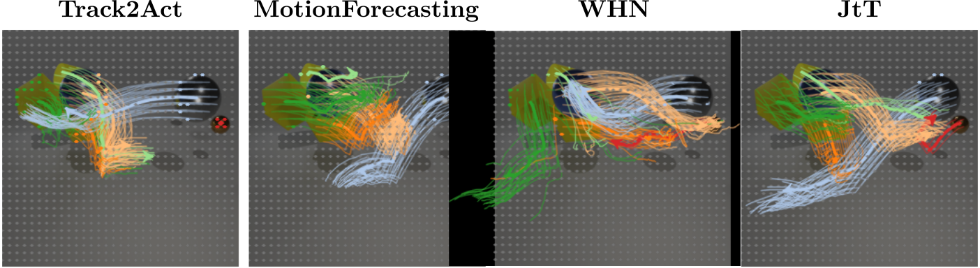
On the Kubric-A benchmark of WHN, every JtT variant improves over all prior trajectory generators on FVMD (D), FVMD (S) and rigidity, with LRTL close to the ground truth.Prior methods are reported at their single published checkpoint, which favors them. GPTF obtains a better Best-of-\(K\), but at the expense of rigidity: its samples are closer to the ground truth pointwise, yet less physically plausible. Methods that diffuse absolute coordinates (Track2Act, WHN, GPTF) obtain poor rigidity, whereas MotionForecasting, the only one diffusing velocities, is the most rigid among them. JtT nevertheless outperforms MotionForecasting on all metrics without using the occlusion labels it requires.
| Model | Size | FVMD (D) | FVMD (S) | Best-of-\(K\) | LRTL |
|---|---|---|---|---|---|
| Ground truth | — | 4,941 | 8,845 | 110.85 | 6.68 |
| Track2Act | 600M | 16,735 | 22,509 | 250.80 | 15.80 |
| WHN (L, latent) | 250M | 13,745 | 17,838 | 127.00 | 14.10 |
| WHN (B, coordinate) | 50M | 14,519 | 18,551 | 137.80 | 23.70 |
| MotionForecasting† | 100M | 20,178 | 26,379 | 186.47 | 8.20 |
| GPTF | 30M* | — | 17,786 | 95.60 | 14.60 |
| JtT-S (Sparse) | 50M | 12,546 (12,238) | 16,769 (16,351) | 160.25 (129.77) | 7.69 (6.91) |
| JtT-B (Sparse) | 200M | 13,514 (11,812) | 17,716 (15,829) | 124.37 (115.24) | 6.67 (6.13) |
| JtT-S (Dense) | 55M | 11,807 (11,591) | 15,695 (15,452) | 135.85 (128.69) | 6.84 (6.64) |
| JtT-B (Dense) | 230M | 13,266 (12,333) | 17,437 (15,958) | 130.44 (118.76) | 6.80 (6.13) |
Sampler
Samples are drawn by solving the SDE with the learned drift via \(1{,}000\) Euler–Maruyama steps and accumulating the predicted velocities. This sampler gives the best rigidity, and needs at least \(250\) steps to be competitive. Euler integration of the probability-flow ODE is robust to the number of steps and achieves similar rigidity with far fewer evaluations.With only \(10\) steps, the ODE sampler improves both FVMD variants and Best-of-\(K\) while using \(100\times\) fewer function evaluations, at the cost of slightly lower rigidity (LRTL \(7.05\) against \(6.77\)).
Results on synthetic data
Each scene below is animated over the \(24\) predicted frames. The top row is the simulated ground truth with four of its futures, followed by four rollouts from JtT-B with the dense and sparse variants, and four rollouts each from WHN, MotionForecasting and Track2Act. Hover a video for the playback controls.
Results on real data
Following WHN, JtT is also trained on real videos from Physics 101, which records simple physical experiments, and on Cityscapes, with identical hyperparameters and training stopped once overfitting is observed on the held-out set.Real videos provide a single observed future per image and no object-level rigidity ground truth, so the rigorous evaluation of the synthetic experiments is not possible here and these results are qualitative. On Physics 101, it generates rigid motion for rigid bodies, such as objects sliding down a ramp or falling onto a table, captures the interaction between rigid and non-rigid bodies, such as a hand releasing an object or a block entering water, and propagates forces through contact.
On Cityscapes, JtT preserves the rigidity of objects that should move rigidly, such as cars, and handles egocentric camera motion well. It generalizes to some extent to deformable objects such as pedestrians, whose overall motion is plausible but less precise than for rigid objects.Cityscapes samples are reasonable but less diverse than on Kubric-A, likely because the model is trained on about \(5\times\) less data: \(2{,}975\) sequences.
Does explicit geometry help?
Oracle geometry from the simulator, as inverse depth at the query points or as queries and trajectories in 3D world coordinates, helps mainly in Best-of-\(K\).For these experiments Kubric-A and Kubric-D are re-rendered with point-to-point correspondence between 2D and 3D trajectories, so absolute numbers differ slightly from the main table. In rigidity, the 2D-only model closes most of the gap between prior 2D methods and the 3D oracle, which supports the design. Integrating monocular 3D reconstruction models is promising future work.
| Input | FVMD (D) | FVMD (S) | Best-of-\(K\) | LRTL (ALL) |
|---|---|---|---|---|
| 2D (ours) | 14,097 | 20,074 | 120.04 | 6.16 |
| 2D + inverse depth | 13,946 | 19,827 | 92.51 | 5.59 |
| 3D world coordinates | 12,909 | 18,518 | 95.02 | 4.37 |
Citation
@article{boduljak2026jtt,
  title   = {JtT: Rethinking Point Trajectory Diffusion for Diverse and Rigid Motion from an Image},
  author  = {Gabrijel Boduljak and Yushi Lan and Christian Rupprecht and Andrea Vedaldi},
  journal = {arXiv preprint},
  year    = {2026}
}